Distributing raster calculations with tiles

Last Update: 7 October 2022
Download Jupyter Notebook: GRWG22_RasterTiles.ipynb

Overview

A common approach to distribute the workload in raster calculations is to split a large raster into smaller ‘tiles’ or ‘chunks’. This tutorial shows how to speed up a NDVI calculation by creating tiles and then distributing the tiles across cores. This process is not specific to calculating NDVI. You can use this approach with any calculation that is performed per cell/pixel without depending on the data in neighboring pixels (if neighboring data is needed, extra steps are involved).

In this tutorial, parallelization is performed within python using the resources allocated to the launched JupyterLab Server session. If you are interested in seeing an example on how to submit your own SLURM job, please see this tutorial.

Language: Python

Primary Libraries/Packages:

Name	Description	Link
rioxarray	rasterio xarray extension	https://corteva.github.io/rioxarray/stable/readme.html
rasterio	access to geospatial raster data	https://rasterio.readthedocs.io/en/latest/
multiprocessing	Process-based parallelism	https://docs.python.org/3/library/multiprocessing.html
dask	Scale the Python tools you love	https://www.dask.org

Nomenclature

• Parallel processing: Distributing computational tasks among multiple cores.
• Core: A processor on a central processing unit; a physical or logical component that can execute computational tasks.
• Tile (or chunk): A continuous segment of a raster dataset or multi-dimensional array.
• NDVI: Normalized Difference Vegetation Index, a quantity derived from the red and near-infrared bands of imagery to detect vegetation.

Analysis Steps

• Open Imagery and Setup Tiles - Open a GeoTIFF of Landsat 7 imagery and divide it into multiple smaller images.
• Define NDVI function - Write a function to calculate Normalized Difference Vegetation Index from an image file.
• Compare serial versus parallel computation times - Measure the time it takes to perform the NDVI calculation across tiles in serial and in parallel
  • Option 1: using the multiprocessing package
  • Option 2: using Dask
• Visualize NDVI results - View the NDVI values in tiles as a whole image.

Step 0: Import Libraries / Packages

Below are commands to run to create a new Conda environment named ‘geoenv’ that contains the packages used in this tutorial series. To learn more about using Conda environments on Ceres, see this guide. NOTE: If you have used other Geospatial Workbook tutorials from the SCINet Geospatial Research Working Group Workshop 2022, you may have aleady created this environment and may skip to launching JupyterHub.

First, we allocate resources on a compute (Ceres) or development (Atlas) node so we do not burden the login node with the conda installations.

On Ceres:

salloc

On Atlas (you will need to replace yourProjectName with one of your project’s name):

srun -A yourProjectName -p development --pty --preserve-env bash

Then we load the miniconda conda module available on Ceres and Atlas to access the Conda commands to create environments, activate them, and install Python and packages.

salloc
module load miniconda
conda create --name geoenv
source activate geoenv
conda install geopandas rioxarray rasterstats plotnine ipython ipykernel dask dask-jobqueue -c conda-forge

To have JupyterLab use this conda environment, we will make a kernel.

ipython kernel install --user --name=geo_kernel

This tutorial assumes you are running this python notebook in JupyterLab. The easiest way to do that is with Open OnDemand (OoD) on Ceres or Atlas. Select the following parameter values when requesting a JupyterLab app to be launched depending on which cluster you choose. All other values can be left to their defaults. Note: on Atlas, we are using the development partition so that we have internet access to download files since the regular compute nodes on the atlas partition do not have internet access.

Ceres:

• Slurm Partition: short
• Number of hours: 1
• Number of cores: 16
• Memory required: 24G
• Jupyer Notebook vs Lab: Lab

Atlas:

• Partition Name: development
• QOS: normal
• Number of hours: 1
• Number of tasks: 16
• Additional Slurm Parameters: –mem=24G

To download the python notebook file for this tutorial to either cluster within OoD, you can use the following lines in the python console:

import urllib.request
tutorial_name = 'GRWG22_RasterTiles.ipynb'
urllib.request.urlretrieve('https://geospatial.101workbook.org/tutorials/' + tutorial_name, 
                           tutorial_name)

Once you are in JupyterLab with this notebook open, select your kernel by clicking on the Switch kernel button in the top right corner of the editor. A pop-up will appear with a dropdown menu containing the geo_kernel kernel we made above. Click on the geo_kernel kernel and click the Select button.

import time
import xarray
import rioxarray
import glob
import os
import rasterio
from rasterio.enums import Resampling
import multiprocessing as mp
from dask.distributed import Client
from dask_jobqueue import SLURMCluster

Step 1a: Open imagery

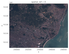
The imagery file we will use is available from the stars R package. It is an example image from Landsat 7. In its documentation, it indicates that the first three bands are from the visible part of the electromagnetic spectrum (blue, green, red) and the fourth band in the near-infrared band. We can use rioxarray’s function open_rasterio to read the imagery file. The plot.imshow function will let us visualize the image in typical RGB. We can see that it is of a coast with forested areas that should have relatively high NDVI values.

L7_ETMs = rioxarray.open_rasterio('https://geospatial.101workbook.org/ExampleGeoWorkflows/assets/L7_ETMs.tif').astype('int16')

# RGB Image using the third-first bands
L7_ETMs[[2,1,0]].plot.imshow()

This image is fairly small and we do not actually need to speed-up the NDVI calculation with parallel processing. So we will make it artificially a big data problem by disaggregating the pixels, i.e. making a greater number of smaller cells, for the sake of a portable example. The function rio.reproject accepts a raster object and a new shape, i.e. a new set of counts for rows and columns. Below, we are using a factor of 20 to disaggregate our raster which will create 400x pixels than the original.

disagg_factor = 20
new_width = L7_ETMs.rio.width * disagg_factor
new_height = L7_ETMs.rio.height * disagg_factor

nir_red_fine = L7_ETMs[[2,3]].rio.reproject(
    L7_ETMs.rio.crs,
    shape=(new_height, new_width),
    resampling=Resampling.nearest,
)

# Save to file
nir_red_fine.rio.to_raster('nr_fine.tif')

Step 1b: Making tiles

First, we will specify how many tiles we want. This example will use 4 tiles in each directions for a total of 16 tiles. Next, we will use nested for loops to iterate through our rows and columns of tiles, subset our fine-scale image to that region, and then write the tile to a file with the tile indices indicated in the filename.

num_tiles = [4,4]

tile_width = int(new_width/num_tiles[0])
tile_height = int(new_height/num_tiles[1])

for i in range(num_tiles[0]):
    for j in range(num_tiles[1]):
        nir_red_tile = nir_red_fine[:,(i*tile_width):((i+1)*tile_width),(j*tile_height):((j+1)*tile_height)]
        nir_red_tile.rio.to_raster('tile_{0}_{1}.tif'.format(i,j))

Step 2: Defining NDVI function

Next, we want to define a function that will calculate NDVI for the pixels in one tile. The function will accept a tile’s filename, open that file with rioxarray, calculate NDVI for the pixels, then write the resulting single-band raster to a new file.

def normalized_diff_r(fname):
  nr = rioxarray.open_rasterio(fname)
  NDVI_r = (nr[1] - nr[0])/(nr[1] + nr[0])
  NDVI_r.rio.to_raster('NDVI_' + fname)

Step 3: Comparing serial and parallel processing times

To have a baseline to which to compare how long the parallel approach takes, we can first time the serial approach. The time.time() function provides basic time reporting capabilities and when called before and after a computation, we can find the processing time as the difference in number of seconds.

Step 3a: multiprocessing

Serial

For our serial approach, we will use a for loop to iterate over our tile files and call our normalized_diff_r function.

tile_files = glob.glob('tile*.tif')
tile_files = [os.path.basename(t_f) for t_f in tile_files]

st = time.time()
for t_f in tile_files:
    normalized_diff_r(t_f)
    
et = time.time()
print('Processing time: {:.2f} seconds'.format(et - st))

Processing time: 7.97 seconds

Parallel

To modify the serial approach above, we can use the multiprocessing function Pool to set how many cores we want to use (here, matching the number of tiles) and the pool.map_async function to asynchonously execute normalized_diff_r for our tiles across those cores.

st = time.time()
pool = mp.Pool(num_tiles[0]*num_tiles[1])
results = pool.map_async(normalized_diff_r, tile_files)
pool.close()    
pool.join()
et = time.time()

print('Processing time: {:.2f} seconds'.format(et - st))

Processing time: 3.23 seconds

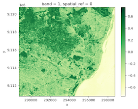
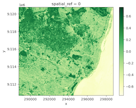
Step 4: Visualize results

We have processed each tile, so we can merge the results back and see our NDVI results.

ndvi_files = ['NDVI_' + t_f for t_f in tile_files]
elements = []
for file in ndvi_files:
    elements.append(rioxarray.open_rasterio(file))

merged = xarray.combine_by_coords(elements).squeeze()

merged.plot.imshow(cmap='YlGn')

Step 5: Parallel - Dask

Dask is an alternative approach to this problem. The package rioxarray, which we used to open our original raster, is a geospatial extension of xarray, a package for manipulating multi-dimensional arrays that also has built-in connections with Dask, a flexible library for parallel computating in Python. We can use the xarray/Dask integration to have the tiling work done for us.

First, we will tell Dask that we are on a cluster managed by SLURM and pass a few arguments to tell SLURM what kind of specification we need. Note that you will need to change yourProjecName name to one of your project’s names.

cluster = SLURMCluster(cores=2, memory='30GB', account='yourProjectName', processes=1)

Since we may not need the same number of cores throughout our processing, or we are not quite sure what the optimal number of cores may be, we can take advantage of Dask’s option to have an adaptive cluster. The code chunk below tells Dask to request from SLURM 1 to 16 jobs at a given time depending on what we request Dask to calculate.

cluster.adapt(minimum_jobs=1, maximum_jobs=16)
client = Client(cluster)

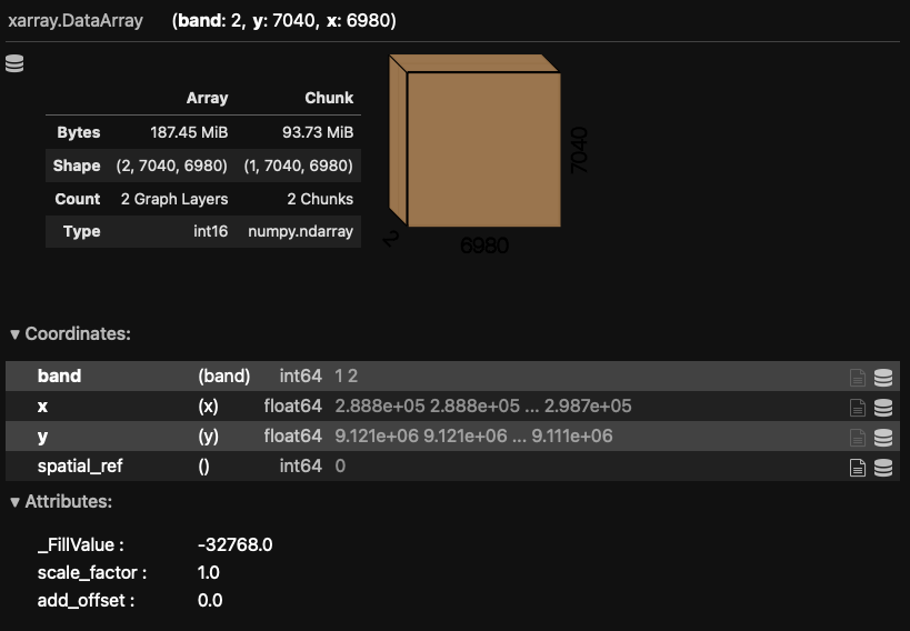
To begin using Dask in our NDVI calculation, we will restart by opening our fine-resolution imagery with rioxarray.open_rasterio, but this time pass a value to the chunks argument. By indicating that we want chunks, we are telling xarray/Dask to split up our multi-dimensional array (multi-band image) into chunks, or tiles. If you are not sure how to define the size of your chunks, you can just pass 'auto' like below and Dask will determine the chunk sizes for you.

When you print the Dask array object information to screen, the chunk sizes (in shape and bytes) are displayed along with a visual of your multi-dimensional array shape and the typical xarray printed information.

L7_ETMs_fine = rioxarray.open_rasterio('nr_fine.tif', chunks= 'auto')
L7_ETMs_fine

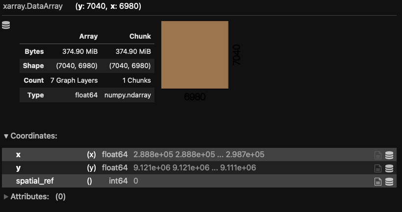
So now we have our imagery open and our chunks defined, we can continue writing our code as we would operate on a typical rioxarray object. The key difference is that Dask arrays defer computation until needed. So we can execute the line below to calculate NDVI for the whole image, but only the instructions are stored - the actual calculation has not happened yet. We print the newly created object and see the Dask-format printed output indicating that the result is now a single band, as we expect for NDVI. That is because Dask is keeping track of how our multi-dimensional array will be modified.

NDVI =  (L7_ETMs_fine[1] - L7_ETMs_fine[0])/(L7_ETMs_fine[1] + L7_ETMs_fine[0])
NDVI

To have the actual calculation be performed, a function requiring the results needs to be called. This can be an explicit request, e.g. the compute function below, or implicit, e.g. plotting the array’s values. Below, we request for our NDVI array to be computed and measure the processing time.

st = time.time()
NDVI.compute()
et = time.time()
print('Processing time: {:.2f} seconds'.format(et - st))

Processing time: 13.72 seconds

During the computation, you can check the SLURM queue by running the squeue -u firstname.lastname in a shell with your SCINet username and see the jobs Dask submits to perform the calculation.

NDVI.plot.imshow(cmap='YlGn')

Continue to explore

Things you can change in this tutorial to see how it affects the difference in processing time between serial and parallel (or the two parallel library options):

• The disaggregation factor
• The number of tiles
• The number of cores