
Last Update: 7 October 2022
Download RMarkdown: GRWG22_RasterTiles.Rmd
Overview
A common approach to distribute the workload in raster calculations is to split a large raster into smaller ‘tiles’ or ‘chunks’. This tutorial shows how to speed up a NDVI calculation by creating tiles and then distributing the tiles across cores. This process is not specific to calculating NDVI. You can use this approach with any calculation that is performed per cell/pixel without depending on the data in neighboring pixels (if neighboring data is needed, extra steps are involved).
This tutorial assumes you are running this Rmarkdown file in RStudio Server. The
easiest way to do that is with Open OnDemand (OoD) on Ceres
or Atlas.
Select the following parameter values when requesting a RStudio Server
app to be launched depending on which cluster you choose. All other values can
be left to their defaults. Note: on Atlas, we are using the development partition
so that we have internet access to download files since the regular compute nodes
on the atlas partition do not have internet access.
Ceres:
Slurm Partition: shortR Version: 4.2.0Number of cores: 16Memory required: 24G
Atlas:
R Version: 4.1.0Partition Name: developmentQOS: normalNumber of tasks: 16Additional Slurm Parameters: –mem=24G
To download the Rmarkdown file for this tutorial to either cluster within OoD, you can use the following lines:
library(httr)
tutorial_name <- 'GRWG22_RasterTiles.Rmd'
GET(paste0('https://geospatial.101workbook.org/tutorials/',tutorial_name),
    write_disk(tutorial_name))
In this tutorial, parallelization is performed within R using the resources allocated to the launched RStudio Server session. If you are interested in seeing an example on how to submit your own SLURM job, please see this tutorial.
Language: R
Primary Libraries/Packages:
| Name | Description | Link |
|---|---|---|
| terra | Spatial Data Analysis | https://cran.r-project.org/web/packages/terra/index.html |
| foreach | Provides Foreach Looping Construct | https://cran.r-project.org/web/packages/foreach/index.html |
| doParallel | Foreach Parallel Adaptor for the ‘parallel’ Package | https://cran.r-project.org/web/packages/doParallel/index.html |
Nomenclature
- Parallel processing: Distributing computational tasks among multiple cores.
- Core: A processor on a central processing unit; a physical or logical component that can execute computational tasks.
- Tile (or chunk): A continuous segment of a raster dataset or multi-dimensional array.
- NDVI: Normalized Difference Vegetation Index, a quantity derived from the red and near-infrared bands of imagery to detect vegetation.
Analysis Steps
- Open Imagery and Setup Tiles - Open a GeoTIFF of Landsat 7 imagery and divide it into multiple smaller images.
- Define NDVI function - Write a function to calculate Normalized Difference Vegetation Index from an image file.
- Compare serial versus parallel computation times - Measure the time it takes to
perform the NDVI calculation across tiles in serial and in parallel
- Option 1: using the
foreachanddoParallelpackages - Option 2: using the
parallelpackage
- Option 1: using the
- Visualize NDVI results - View the NDVI values in tiles as a whole image.
Step 0: Import Libraries/Packages
For this tutorial, we will use the stars package for one of its example
datasets, the terra package for handling raster data, and the doParallel and
foreach packages together for distributing our calculations. The stars and
terra packages are each available in the R site library for RStudio Server on
Ceres and Atlas Open OnDemand, though not in the R site library if you were to load an R
module in a shell. However, the terra version on Atlas is not a recent enough
version for this tutorial, so we will install the latest version. As of this
writing, foreach and doParallel are not in the
site library and will need to be installed if you have not already done so. To
learn more about installing packages on Ceres, see
this guide.
install.packages(c('foreach','doParallel','terra'))
library(terra)
library(foreach)
library(doParallel)
Step 1: Open Imagery and Setup Tiles
Step 1a: Open imagery
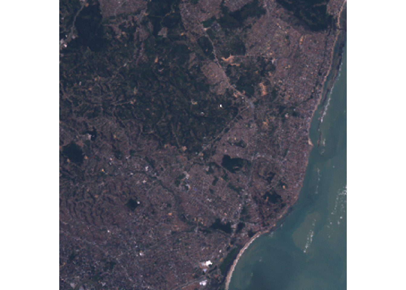
The imagery file we will use is available from the stars package. It is an
example image from Landsat 7 and you can learn more about it by calling
?L7_ETMs. In that documentation, it indicates that the first three bands are
from the visible part of the electromagnetic spectrum (blue, green, red) and the
fourth band in the near-infrared band. We can use terra’s function rast to
read the imagery file. The plotRGB function will let us visualize the image in
typical RGB. We can see that it is of a coast with forested areas that should
have relatively high NDVI values.
L7_ETMs <- rast(system.file("tif/L7_ETMs.tif", package = "stars"))

# RGB Image using the third-first bands
plotRGB(L7_ETMs[[3:1]])
This image is fairly small and we do not actually need to speed-up the NDVI
calculation with parallel processing. So we will make it artificially a big data
problem by disaggregating the pixels, i.e. making a greater number of smaller
cells, for the sake of a portable example. The function disagg accepts a
raster object and a disaggregation factor, i.e. the number of cells to create from
each original cell in each direction. Below, we are using a factor of 20 which
will create 400x pixels than the original.
disagg_factor <- 20
nir_red_fine <- disagg(L7_ETMs[[3:4]], disagg_factor,
                       filename = "nr_test.tif",
                       overwrite = TRUE)
Step 1b: Making tiles
The terra package comes with a handy function for making raster tiles called
makeTiles to which you pass the raster you want to split up, a template raster
indicating how to split it up into tiles, and how to name the resulting files
containing the tiles. First, we will specify how many tiles we want. This example
will use 4 tiles in each directions for a total of 16 tiles. Next, we will create
an empty raster template will the number of rows and columns matching our number
of tiles and our image’s spatial extent and CRS. The we call makeTiles which
will write the tiles to file and return the filenames.
# Set number of tiles (number of rows, number of columns)
num_tiles <- c(4,4)

# Define empty raster template to define tiles
tile_template <- rast(nrows = num_tiles[1],
                      ncols = num_tiles[2],
                      crs = crs(nir_red_fine),
                      ext = ext(nir_red_fine))

# Generate the tile files using the red and NIR bands only
nr_tiles <- makeTiles(nir_red_fine,
                      tile_template,
                      filename="tile_.tif",
                      overwrite=TRUE)
Step 2: Defining NDVI function
Next, we want to define a function that will calculate NDVI for the pixels in
one tile. The function will accept a tile’s filename, open that file with terra,
calculate NDVI for the pixels, then write the resulting single-band raster to
a new file.
# Define NDVI function that writes results to file
normalized_diff_r <- function(fname){
  nr <- rast(fname)
  NDVI_r <- (nr$L7_ETMs_4 - nr$L7_ETMs_3)/(nr$L7_ETMs_4 + nr$L7_ETMs_3)

  writeRaster(NDVI_r, filename=paste0('NDVI_',fname), overwrite = TRUE)
}
Step 3: Comparing serial and parallel processing times
To have a baseline to which to compare how long the parallel approach takes, we
can first time the serial approach. The base R system.time() function provides
basic timing capabilities and reports three different timings: user, system,
and elapsed. The third timing, elapsed, is the physical or ‘wall’ time elapsed
and the one we are interested in comparing among our approaches.
Step 3a: foreach/doParallel
Serial
In this first option, we are using the foreach package as a serial backend that
the doParallel extends with parallel processing. Using foreach is similar to
using a for loop with a slightly different syntax in the first line:
foris replaced withforeachinis replaced with=){is replaced with) %do% {
# for loop
for(i in 1:N){
  # Do your calculation
}

# foreach
foreach(i = 1:N) %do% {
  # Do your calculation
}
To have NDVI calculated for each of our tiles, we will have foreach iterate
over each tile filename (which was returned by makeTiles) and call our
normalized_diff_r function for each iteration.
# Time the serial execution
system.time({
  foreach(fname=nr_tiles) %do% {
    normalized_diff_r(fname)
  }
})
   user  system elapsed
 10.277   0.296  12.665
Parallel
To use doParallel to parallelize foreach, two things must be done:
- You register
doParallelwith the number of cores you want to use - You change
%do%to%dopar%in yourforeachstatement
Here, we are using as many cores as number of tiles so each core will have one task to complete.
# Register doParallel
registerDoParallel(cores = prod(num_tiles))

# Time the parallel execution
system.time({
  foreach(fname=nr_tiles) %dopar% {
    normalized_diff_r(fname)
  }
})
   user  system elapsed
  9.144   1.426   8.189
Step 3b: parallel
There is another similar approach using the parallel package, which comes with
base R. Instead of extending foreach, we will see how parallel extends base
R’s lapply with mclapply.
Serial
Again, we will first time how long the serial lapply approach takes to perform
our NDVI calculation. lapply accepts a vector of inputs (our tile filenames)
and a function that accepts those inputs (normalized_diff_r).
# Time the serial execution
system.time({
  lapply(nr_tiles, normalized_diff_r)
})
   user  system elapsed
 10.302   0.260  12.746
Parallel
To use the parallel version of lapply, two changes are made to our
code above:
- Call
mclapplyinstead oflapply - Pass the desired number of cores
Like with doParallel, we are requesting as many cores as the number of tiles.
# Time the parallel execution
system.time({
  mclapply(nr_tiles, normalized_diff_r, mc.cores = prod(num_tiles))
})
   user  system elapsed
  6.226   1.213   7.670
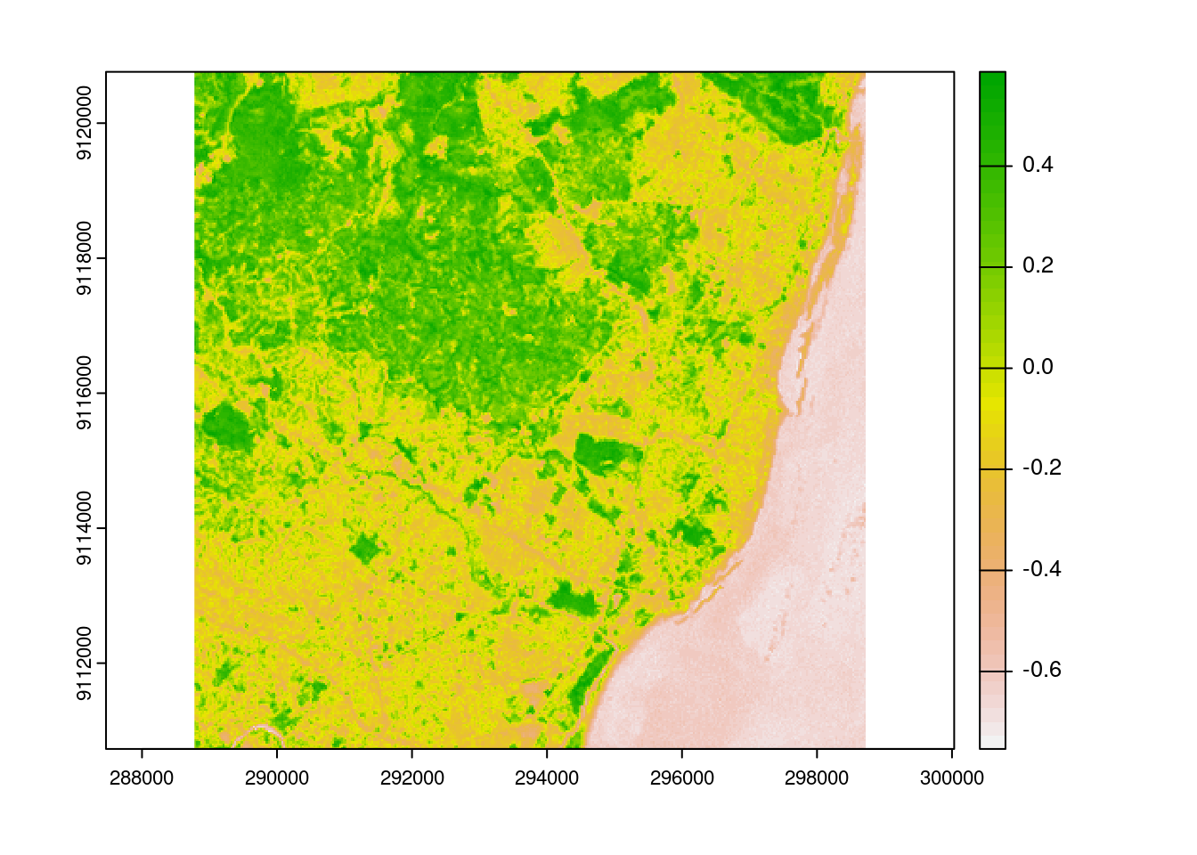
Step 4: Visualize NDVI results
There is a terra function vrt (Virtual Raster Tiles) for visualizing tiles
without having to mosaic first. Note: if you are familiar with using
GDAL (Geospatial Data Abstraction Library), their
VRT is a more general virtual format
not specific to just tiling.
We can see from the image that the forested areas have the higher NDVI values as we expected.
virtual_ndvi <- vrt(paste0('NDVI_',nr_tiles))
plot(virtual_ndvi)
Continue to explore
Things you can change in this tutorial to see how it affects the difference in processing time between serial and parallel (or the two parallel library options):
- The disaggregation factor
- The number of tiles
- The number of cores