```{r setup, include=FALSE}
knitr::opts_chunk$set(
echo = TRUE,
collapse = TRUE,
comment = "#>",
fig.path = "images/R_"
)
```
**Last Update:** 14 Jan 2021
**RMarkdown:** [R_Image_Processing.Rmd](https://geospatial.101workbook.org/tutorials/R_Image_Processing.Rmd)
## Overview
In this tutorial, we present a brief overview of image processing concepts necessary to understand machine learning and deep learning. This walk through was originally written in python: [link to python version](https://geospatial.101workbook.org/Workshops/Tutorial1_Image_Processing_Essentials_Boucheron.html). We have tried to maintain functionality across both languages but certain libraries/features may only be available in one or the other. The basics of image processing should be the same across both.
This tutorial explores:
* Loading image files into R
* Printing properties of an image
* Converting an image between color and grayscale
* Identifying features (edges) within an image
## Downloading Images
We will be using two images which can be downloaded from the following links:
* [cameraman.png](https://geospatial.101workbook.org/Workshops/Tutorial1_Image_Processing_Essentials_Boucheron.html)
* [peppers.png]()
cameraman.png|peppers.png
:-------------------------:|:-------------------------:
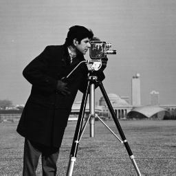 |
| 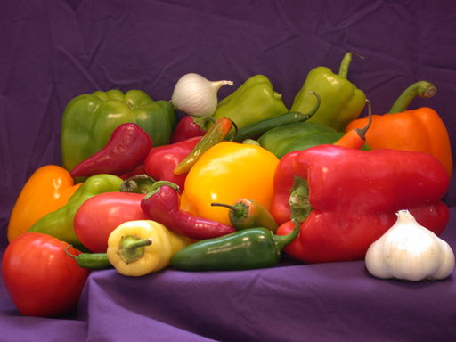 From a terminal, we could have used the `wget` or `curl` commands to download the images.
```{bash, eval=FALSE}
wget https://geospatial.101workbook.org/tutorials/data/cameraman.png
wget https://geospatial.101workbook.org/tutorials/data/peppers.png
ls -1 *.png
#> cameraman.png
#> peppers.png
```
The `cameraman.png` on the left is in grayscale and the `peppers.png` on the right is in color. Processing color or grayscale images is slightly different, which we will explore in the following tutorial.
## Loading images into R
We will assume you have a working R environment; however, see the following for a tutorial on setting up an R environment:
* [Set up R and R Environment](https://bioinformaticsworkbook.org/dataWrangling/R/r-setup.html#gsc.tab=0)
The nice thing about scripting languages is the fact that many tools are published as libraries. Which means you do not have to write your own functions from scratch.
For this tutorial, we will be using R's `imager` library available on CRAN ([link to more info](http://dahtah.github.io/imager/)). There may be other image libraries more suited to your analysis, and we highly encourage you to explore, especially as new libraries are constantly being developed.
Below, we can install and load the `imager` library.
```{r, message=FALSE, warning=FALSE}
# install.packages("imager") # <= uncomment to install from CRAN
library(imager)
```
From there, we can use the `load.image` function to read in `cameraman.png`. You may need the path to your input file, if they are not in the same location.
```{r I_camera}
I_camera = load.image('data/cameraman.png') # <= path to input image here
plot(I_camera)
```
Here, we have read in the image and stored it as `I_camera`. To verify that the image was successfully loaded into R, we have displayed the image using the `plot` function.
From the plot, notice how the x-axis goes from 0 to 300 from left to right. Strangely, the y-axis goes from 0 to 300, top to bottom. Therefore, the xy point (0,0) is actually the **top left** of the image. This can be very important **as your analysis results may be different if the (0,0) is top left, right, bottom, or center**. It's a good idea to check where (0,0) is in the image.
Now, we can also load the `peppers.png` in the same way, and store it as `I_peppers`.
```{r I_peppers}
I_peppers = load.image('data/peppers.png') # <= path to input image here
plot(I_peppers)
```
## Properties of an image
Now that we've loaded and plotted the images. What is an image object and its properties?
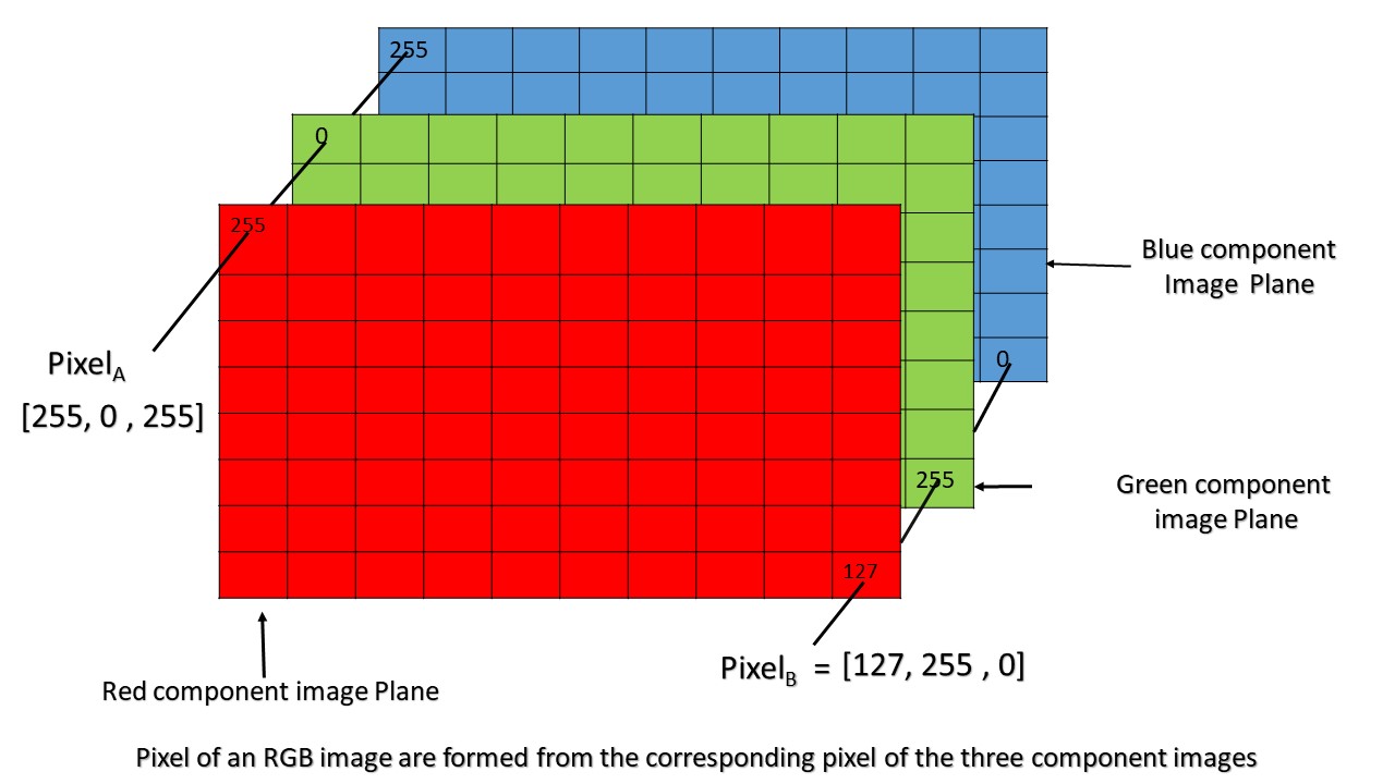
An image is actually stored as a matrix of pixels, usually stored in multiple layers. The diagram from https://media.geeksforgeeks.org/wp-content/uploads/Pixel.jpg is a good illustration of the concept of image layers.
From R, we can look at the structure (`str`) of a variable (`I_camera`) by the following:
```{r}
str(I_camera)
```
The structure of `I_camera` is an array of numbers `cimg num [1:256, 1:256, 1, 1]`. This is showing the dimension of the images to be 256 pixels wide, 256 pixels high, with 1 depth (layer), and 1 channel (because it's a grayscale image).
Now, let's look at `I_peppers`, which is a color image. How is the structure different?
```{r}
str(I_peppers)
```
Other then a 512 pixel width and 384 pixel height, notice how the 4th term is `1:3`
which indicates three channels (RGB or Red Green Blue).
We could have also used the dimension (`dim`) function to quickly compare them.
```{r}
dim(I_camera) # Width_in_pixels Height_in_pixels Depth(layers) color(1=grayscale, 3=RGB)
dim(I_peppers)
```
## Subregions of the image
Since an image object is really an R matrix, the matrix sub setting functions work to subset an image. Here, we pull out a subregion near the center of the image (100 to 110 pixels high and wide) and store it as `sub_I_camera`
```{r sub_I_camera}
sub_I_camera = as.cimg(I_camera[100:110,100:110,,] )
plot(sub_I_camera)
```
From this smaller `sub_I_camera`, we can print out the pixel values, get the minimum value and maximum value.
```{r}
sub_I_camera[,,,1]
min(sub_I_camera[,,,1])
max(sub_I_camera[,,,1])
```
See if you can subset and explore the `I_peppers` color image. Try to pull out a subimage that only contains one pepper.
## Convert to Color Images to Grayscale
There are many reasons why we might want to convert a color image to a grayscale image. For one thing, it results in a reduction in image size (drop the 3 channels into 1). Another reason, is we want to focus on one color to identify an object in a busy scene. Or we may want to flatten certain layers to better identify edges of an object of interest.
Recall the `I_peppers` color image?
```{r I_pepper}
I_peppers = load.image('data/peppers.png') # <= path to peppers.png
plot(I_peppers)
```
The `imager` package provides a convenient `grayscale` function.
```{r gray_I_peppers}
gray_I_peppers = grayscale(I_peppers)
plot(gray_I_peppers)
```
Recall that an image is really a matrix of numbers. Let's compare the dimensions of the original with the new image.
```{r}
dim(I_peppers) # Color Original
dim(gray_I_peppers) # Grayscale Transformed
```
The only difference should be the 4th entry.
## Identify edge features in an image.
In order to identify objects in an image, it is often necessary to identify edges. While humans can intuitively identify edges to an object, computational edge detection is a bit more noisy. Usually it involves defining some gradiant function. An example shown below:
```{r edge_I_camera}
dx <- imgradient(I_camera, "x")
dy <- imgradient(I_camera, "y")
grad.mag <- sqrt(dx^2 + dy^2)
plot(grad.mag, main="Gradient magnitude")
```
This particular function is called a Sobal Filter. To read more about Sobal filters, see this link: [wikipedia - sobel operator](https://en.wikipedia.org/wiki/Sobel_operator)
What happens if we identify edges in the color image `I_peppers`?
```{r edge_I_peppers}
dx <- imgradient(I_peppers, "x")
dy <- imgradient(I_peppers, "y")
grad.mag <- sqrt(dx^2 + dy^2)
plot(grad.mag, main="Gradient magnitude")
```
What happens if we convert the color image to a gray scale image first?
```{r edge2_I_peppers}
gray_I_peppers = grayscale(I_peppers)
dx <- imgradient(gray_I_peppers, "x")
dy <- imgradient(gray_I_peppers, "y")
grad.mag <- sqrt(dx^2 + dy^2)
plot(grad.mag, main="Gradient magnitude")
```
# In summary
Hopefully you have learned how to:
* load image files into R,
* identify the dimensions of the image (gray vs color),
* learned some common transformations (pull out subregions, convert to grayscale),
* and identify edge features.
These colors and features can be fed into Machine Learning algorithms for image recognition such as but not limited to identifying roadways, forest cover, and snow cover. Hopefully, this has provided you with some intuition on how to perform analysis/transformations on image files.
From a terminal, we could have used the `wget` or `curl` commands to download the images.
```{bash, eval=FALSE}
wget https://geospatial.101workbook.org/tutorials/data/cameraman.png
wget https://geospatial.101workbook.org/tutorials/data/peppers.png
ls -1 *.png
#> cameraman.png
#> peppers.png
```
The `cameraman.png` on the left is in grayscale and the `peppers.png` on the right is in color. Processing color or grayscale images is slightly different, which we will explore in the following tutorial.
## Loading images into R
We will assume you have a working R environment; however, see the following for a tutorial on setting up an R environment:
* [Set up R and R Environment](https://bioinformaticsworkbook.org/dataWrangling/R/r-setup.html#gsc.tab=0)
The nice thing about scripting languages is the fact that many tools are published as libraries. Which means you do not have to write your own functions from scratch.
For this tutorial, we will be using R's `imager` library available on CRAN ([link to more info](http://dahtah.github.io/imager/)). There may be other image libraries more suited to your analysis, and we highly encourage you to explore, especially as new libraries are constantly being developed.
Below, we can install and load the `imager` library.
```{r, message=FALSE, warning=FALSE}
# install.packages("imager") # <= uncomment to install from CRAN
library(imager)
```
From there, we can use the `load.image` function to read in `cameraman.png`. You may need the path to your input file, if they are not in the same location.
```{r I_camera}
I_camera = load.image('data/cameraman.png') # <= path to input image here
plot(I_camera)
```
Here, we have read in the image and stored it as `I_camera`. To verify that the image was successfully loaded into R, we have displayed the image using the `plot` function.
From the plot, notice how the x-axis goes from 0 to 300 from left to right. Strangely, the y-axis goes from 0 to 300, top to bottom. Therefore, the xy point (0,0) is actually the **top left** of the image. This can be very important **as your analysis results may be different if the (0,0) is top left, right, bottom, or center**. It's a good idea to check where (0,0) is in the image.
Now, we can also load the `peppers.png` in the same way, and store it as `I_peppers`.
```{r I_peppers}
I_peppers = load.image('data/peppers.png') # <= path to input image here
plot(I_peppers)
```
## Properties of an image
Now that we've loaded and plotted the images. What is an image object and its properties?
An image is actually stored as a matrix of pixels, usually stored in multiple layers. The diagram from https://media.geeksforgeeks.org/wp-content/uploads/Pixel.jpg is a good illustration of the concept of image layers.

From R, we can look at the structure (`str`) of a variable (`I_camera`) by the following:
```{r}
str(I_camera)
```
The structure of `I_camera` is an array of numbers `cimg num [1:256, 1:256, 1, 1]`. This is showing the dimension of the images to be 256 pixels wide, 256 pixels high, with 1 depth (layer), and 1 channel (because it's a grayscale image).
Now, let's look at `I_peppers`, which is a color image. How is the structure different?
```{r}
str(I_peppers)
```
Other then a 512 pixel width and 384 pixel height, notice how the 4th term is `1:3`
which indicates three channels (RGB or Red Green Blue).
We could have also used the dimension (`dim`) function to quickly compare them.
```{r}
dim(I_camera) # Width_in_pixels Height_in_pixels Depth(layers) color(1=grayscale, 3=RGB)
dim(I_peppers)
```
## Subregions of the image
Since an image object is really an R matrix, the matrix sub setting functions work to subset an image. Here, we pull out a subregion near the center of the image (100 to 110 pixels high and wide) and store it as `sub_I_camera`
```{r sub_I_camera}
sub_I_camera = as.cimg(I_camera[100:110,100:110,,] )
plot(sub_I_camera)
```
From this smaller `sub_I_camera`, we can print out the pixel values, get the minimum value and maximum value.
```{r}
sub_I_camera[,,,1]
min(sub_I_camera[,,,1])
max(sub_I_camera[,,,1])
```
See if you can subset and explore the `I_peppers` color image. Try to pull out a subimage that only contains one pepper.
## Convert to Color Images to Grayscale
There are many reasons why we might want to convert a color image to a grayscale image. For one thing, it results in a reduction in image size (drop the 3 channels into 1). Another reason, is we want to focus on one color to identify an object in a busy scene. Or we may want to flatten certain layers to better identify edges of an object of interest.
Recall the `I_peppers` color image?
```{r I_pepper}
I_peppers = load.image('data/peppers.png') # <= path to peppers.png
plot(I_peppers)
```
The `imager` package provides a convenient `grayscale` function.
```{r gray_I_peppers}
gray_I_peppers = grayscale(I_peppers)
plot(gray_I_peppers)
```
Recall that an image is really a matrix of numbers. Let's compare the dimensions of the original with the new image.
```{r}
dim(I_peppers) # Color Original
dim(gray_I_peppers) # Grayscale Transformed
```
The only difference should be the 4th entry.
## Identify edge features in an image.
In order to identify objects in an image, it is often necessary to identify edges. While humans can intuitively identify edges to an object, computational edge detection is a bit more noisy. Usually it involves defining some gradiant function. An example shown below:
```{r edge_I_camera}
dx <- imgradient(I_camera, "x")
dy <- imgradient(I_camera, "y")
grad.mag <- sqrt(dx^2 + dy^2)
plot(grad.mag, main="Gradient magnitude")
```
This particular function is called a Sobal Filter. To read more about Sobal filters, see this link: [wikipedia - sobel operator](https://en.wikipedia.org/wiki/Sobel_operator)
What happens if we identify edges in the color image `I_peppers`?
```{r edge_I_peppers}
dx <- imgradient(I_peppers, "x")
dy <- imgradient(I_peppers, "y")
grad.mag <- sqrt(dx^2 + dy^2)
plot(grad.mag, main="Gradient magnitude")
```
What happens if we convert the color image to a gray scale image first?
```{r edge2_I_peppers}
gray_I_peppers = grayscale(I_peppers)
dx <- imgradient(gray_I_peppers, "x")
dy <- imgradient(gray_I_peppers, "y")
grad.mag <- sqrt(dx^2 + dy^2)
plot(grad.mag, main="Gradient magnitude")
```
# In summary
Hopefully you have learned how to:
* load image files into R,
* identify the dimensions of the image (gray vs color),
* learned some common transformations (pull out subregions, convert to grayscale),
* and identify edge features.
These colors and features can be fed into Machine Learning algorithms for image recognition such as but not limited to identifying roadways, forest cover, and snow cover. Hopefully, this has provided you with some intuition on how to perform analysis/transformations on image files.